Short-term demand forecasting guide

When planning inventory levels, demand planners often face a critical tradeoff: using simple forecasting methods that are easy to implement or investing in sophisticated AI-powered approaches that deliver superior accuracy. Basic methods like moving averages can keep costs low and provide quick results. However, they often miss complex patterns, seasonal variations and market changes that lead to costly stockouts or excess inventory.

Alternatively, advanced AI models can improve short-term demand forecasting accuracy by up to 55%, but they require significant data preparation, technical expertise and ongoing maintenance.

Sources: Comparative Analysis of Traditional and AI-based Demand Forecasting Models, International Journal of Emerging Trends in Science and Technology; STX Next Machine Learning in Forecasting vs. Traditional Methods

This guide will help you choose the right forecasting approach by comparing six proven methods, explaining data requirements and showing you how 3PL partners like Cart.com eliminate forecasting complexity while delivering enterprise-grade accuracy.

Method analysis: Deep-dive into each forecasting approach

Moving average: The foundational method

Moving averages make up the industry standard for short-term demand forecasting, allowing teams to calculate demand by averaging recent historical periods. For example: 

This makes them perfect for stable demand forecasting without significant seasonality. Beyond that, they’re simple to implement and understand, which is why even high-level 3PLs like Cart.com use them as baseline calculations in their inventory and demand forecasting AI platform.

Best for: Mature products with consistent demand, basic inventory planning and quick forecasting when resources are limited.

Exponential smoothing: Trend-aware forecasting

Exponential smoothing operates on the idea that recent observations should have more influence on future predictions than older ones. Moreover, the relative weight of older predictions should decrease as they get older. 

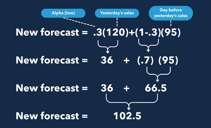
A simple explanation of how exponential smoothing works would look something like this:

New forecast=a(latest value)+(1-a)(previous forecast)

In this formula, “a” refers to “alpha,” a smoothing constant between 0 and 1. What does this mean? The higher the “alpha,” the more responsive the formula will be to recent changes, whereas a lower alpha is more stable and less reactive to fluctuations.

When applied to something simple like an ecommerce shop, the formula would look like this: 

Advanced versions, such as Holt-Winters, handle both trends and seasonality, which Cart.com integrates into its AI forecasting engine for products showing clear seasonal patterns.

Best for: Products with trending patterns, seasonal items with predictable cycles and mid-range complexity forecasting needs.

ARIMA models: Statistical sophistication

Autoregressive integrated moving average (ARIMA) is a sophisticated statistical forecasting method that combines autoregression (using past values), differencing (removing trends) and moving averages (smoothing errors) to model complex time series data. It’s designed to handle non-stationary data that exhibits trends, seasonality and other temporal patterns.

While statistically robust, they require expertise to implement properly. Take the following example: 

To start, an ARIMA method would note the existing trends in the dataset. For example: 

• Year 2 numbers are ~10 points higher than year 1

• Summer months tend to show higher sales

Following this analysis, it would then calculate changes from one period to the next: 

Notably, the variances in this dataset are identical in both years, suggesting normalized demand fluctuation throughout the year to accompany the steady growth noted in step 1. The company’s fulfillment needs are growing, not peaking. 

With the differencing complete, teams will then use the autocorrelation function (ACF) and/or partial autocorrelation function (PACF) parameters to find the optimal ARIMA values for the data, which can then be fit into statistical software. In the case of our ecommerce shop from before, the analysis would likely identify an ARIMA(1,1,1) model, meaning:

• 1 autoregressive term (current forecast depends on the previous month’s change)
• 1 degree of differencing (the trend removal we just completed)
• 1 moving average term (incorporates previous forecast errors)

To forecast month 25 (January of year 3), the model would calculate:

• Previous change: December sales dropped 5 units from November
• Expected January change: 0.3 × (-5) = -1.5 units
• January forecast: 135 + (-1.5) = 133.5 thousand units

For month 26, the pattern continues but with diminishing influence:

• Expected February change: 0.3 × (-1.5) = -0.45 units
• February forecast: 133.5 + (-0.45) = 133.05 thousand units

While ARIMA models are standard in time studies, the reality of calculation makes them particularly difficult to do by hand. Working with an experienced party like a 3PL or dedicated logistics personnel tends to be the default means of implementation for companies seeking ARIMA-level forecasting, since they provide clients with clean, transparent, visible and accurate data that removes the strain from making ARMIA calculations manually.

Best for: Complex seasonal patterns, products with rich historical data and situations requiring statistical rigor.

Random forest machine learning: Multi-variable intelligence

Random forest builds multiple decision trees using different data subsets, then averages predictions for robust forecasting. It excels at capturing non-linear relationships between variables, which makes it a core component of Cart.com’s machine learning stack.

While powerful at pattern recognition, they require substantial data preparation and computational resources. Take the following example:

To start, a Random Forest model would create 100+ individual decision trees, each trained on random subsets of this historical data and containing their own unique decision rules. For example:

• • Tree 1 might focus on marketing spend, temperature and review scores
    • If marketing_spend > $50K and review_score > 4.2, predict 2,950 units
    • If marketing_spend ≤ $50K and temperature < 70°F, predict 2,400 units

• • Tree 2 could emphasize competitor pricing, unemployment and seasonality
    • If competitor_price_ratio > 1.2 and unemployment > 4.1%, predict 2,100 units
    • If competitor_price_ratio ≤ 1.2 and back_to_school = 1, predict 3,200 units

As the team looks at the January forecast, each tree processes these inputs through its unique decision rules:

• Tree 1:
  • Marketing > $50K (yes)
  • Review score > 4.2 (no)
    • Follows alternate path → predicts 2,650 units
• Tree 2:
  • Competitor ratio > 1.2 (no)
  • Back-to-school = 0 

Continuing through all 100 trees:

• • Tree 1-25 average: 2,680 units
  • Tree 26-50 average: 2,590 units
  • Tree 51-75 average: 2,720 units
  • Tree 76-100 average: 2,610 units

This results in the final random forest prediction: (2,680 + 2,590 + 2,720 + 2,610) ÷ 4 = 2,650 units

Of the short-term demand forecasting options, random forest machine learning provides exceptional predictive power, stability and ability for adaptation in the face of missing data. However, this sophistication comes with computational demands and interpretability challenges. 

• Unlike simple averages that anyone can verify, random forest predictions emerge from hundreds of complex decision trees that even experts struggle to fully explain. 
• The model also requires continuous feature engineering to transform raw business data into meaningful predictor variables that trees can utilize effectively.

Best for: Multi-channel environments, products influenced by external factors and mid-to-large operations with diverse data sources.

Neural networks: Deep learning power

Neural networks, especially long short-term memory (LSTM) networks, identify complex patterns in large datasets with exceptional accuracy. They require significant data and computational power but deliver superior results. Take the following example:

To understand how neural network forecasting works, consider the following dataset:

An LSTM neural network would process this data through multiple interconnected layers, each designed to recognize different types of patterns:

Each LSTM cell processes information through specialized gates that control memory:

• Forget gate: What to forget (Ex.“Temperature from 60 days ago isn’t relevant”)

• Input gate: What to remember (Ex. “Holiday effect + high marketing = important”)

• Output gate: What to use now (Ex. “Recent weather trend + social buzz = predict higher”)

With the parameters set, the LSTM analyzes the new data for day 91:

What makes neural networks exceptionally powerful is their ability to learn complex, non-linear relationships that traditional methods miss; their memory capabilities allow them to recognize that current conditions (hot weather + holiday + high marketing) create a unique combination that occurred only twice in the training data, both resulting in 24,000+ unit sales days.

The learning ability of neural network systems is best exemplified in their backpropagation training, one of several learning algorithms that continuously refines their understanding for the purpose of making future predictions:

The sophistication of neural network demand forecasting requires enormous computational resources. They also suffer from “black box” opacity. While the 94% accuracy is impressive, business leaders cannot easily understand which specific factors drove the prediction or validate the reasoning behind unusual forecasts.

Best for: Large product catalogs, dynamic pricing environments and high-volume operations requiring precise accuracy.

Understanding the tradeoff: Accuracy vs complexity

As the short-term demand forecasting methods above imply, evaluating your own forecasting is a process of balancing accuracy vs complexity. To make things difficult, there are reasons to choose both:

This challenge is especially true when considering what kind of data you have available. Regardless of your choice of short-term demand forecasting, poor data quality kills forecasting accuracy, even with sophisticated AI. Common problems include inconsistent product hierarchies, missing seasonal adjustments, absent external factor data and stockouts recorded as zero demand rather than lost sales.

The following rubric can help you score your own data quality, for reference.

Balancing accuracy and complexity can be challenging because delivering precise forecasts may require significant investment in data infrastructure, technical talent and computational resources. But with Cart.com’s AI-powered forecasting, you don’t have to choose between the two.

Enacting a short-term demand forecasting strategy

Advanced short-term demand forecasting requires balancing technical sophistication with practical constraints. While traditional methods offer simplicity, modern AI approaches can deliver up to 55% accuracy improvements through hybrid methodologies.

The complexity of managing data quality, feedback loops and multi-variable optimization creates significant operational challenges. This is precisely where specialized 3PL providers excel, eliminating forecasting complexity while improving accuracy across your entire supply chain.

Reach out for an initial conversation with a representative to discover how an AI-powered demand forecasting can transform your inventory management.